By Chi-An Wang, Dailin Shen=
Threshold Test Model
We believe the threshold test is a better model compared to the benchmark test and the outcome test. The benchmark test has the qualified pool problem that might overlook the case that the officers are doing good policing. The outcome test also has the problem of infra-marginality problem that might speculate discrimination while there is not. These two model have the advantage of easier to compute and intuitiveness but might neglect some of the key features in the process of policing.
Why do we think threshold test is a fair metric?
Being bias is having a double standard, and threshold test well mapped this concept to having a lower threshold of deciding to search the stopped driver. Simoiu added two important features, the subjective probabilities, and search threshold, as a latent variable into the threshold test model. The subjective probabilities p (the officers feeling about the driver possessing contraband) is drawn from a binomial distribution parameterized by 1. Phi_{rd} and lambda_{rd}. Phi_{rd} models the probability that a driver is carrying contraband and lambda express the difficulty in distinguishing between guilty and innocent drivers. The threshold is the most important latent variables inferred from data so that we can compare between different race.
This modeling makes sense since it models the real-world process of P making decisions. Rather than only based on the stop and frisk results, they assume that how the people reacted to the police and its appearance would also be taken into consideration into the beta distribution. It also takes the difference between each precinct into consideration.
Although Police making a calibrated decision might not be totally realistic, but we would argue that the data that we’re modeling is a single year dataset of 2011. The long-term variation in this year might not be huge. For example, a young police might not be tough until working for several years while an old police might not change its way of policing after 30 years.
Data Preprocessing – iPython Notebook
1 Contraband
The paper “Testing for Racial Discrimination in Police Searches of Motor Vehicles” categorized four types of contrabands, including drugs, alcohol, weapons, and money. While, the description in the file specifications of the database ( NYPD Stop Question Frisk Database 2015) only showed a single type of contraband, which was the weapon. Also, we found the database concentrated more on different kinds of weapons, like rifles, pistols, assault weapons and knife cuttings. Hence we decided to use these four types of weapons as one of our proxies to prediction.
2 Race
There are eight different races in our dataset, which includes A(“Asian/Pacific Islander”), B(“Black”), I(“American Indian/Alaskan Native”), P(“Black-Hispanic”), Q(“White-Hispanic”), W(“White”), X(“Unknown”), Z(“Other”). We decided to merge Black-Hispanic and White-Hispanic based on the assumption that people in the States, especially the officers, are capable of telling them apart from Black and White. Therefore to provide a slightly bigger dataset and make good use of them, we decided to merge them and drop all other smaller races.
3 Age
We noticed that the age in our dataset ranged from 0 to 999, although most of the ages clustered obeyed the normal distribution. To let calculation make more sense, according to news publications, we found that the longest age in the USA is 116, hence we omitted the observations with the age over 116.
Benchmark
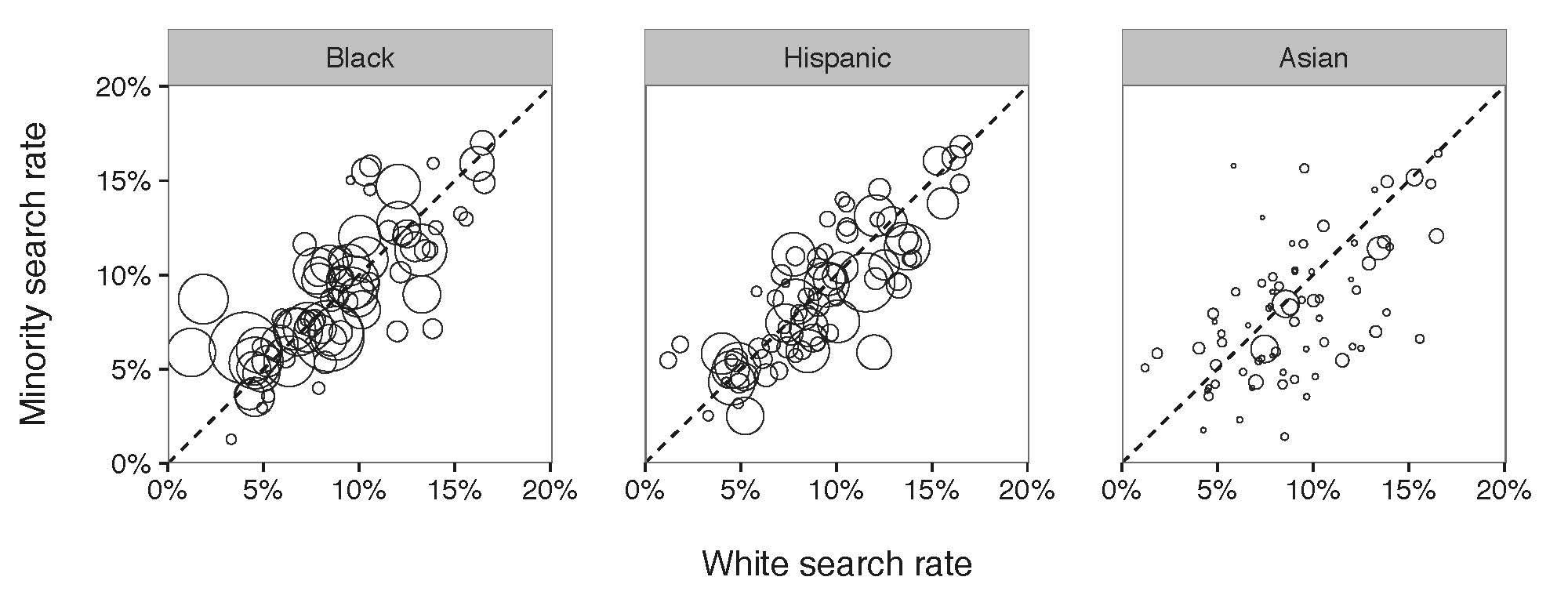
Figure 1: Results of benchmark on a department-by-department basis. Each circle in the diagram refers to a police department and the affiliated search rate of minority compared to White search rate.
The X-axis in Figure 1 is the observed White search rate, and, the Y-axis is the observed Minority search rate. Each point in the diagram compares search rates of minority and white drivers for a single department. The size of a point illustrates the number of drivers being stopped by the department. We expect to see all the points locating on the diagonal line if there is no discrimination against minorities. Otherwise, if all the points locate above the diagonal line, a discrimination exists; if all the points locate below the diagonal line, there is no discrimination . According to Figure 1, so far, we incline to say that there is a slightly discrimination against Black and slightly group, but no clear discrimination against Asian drivers.
Outcome
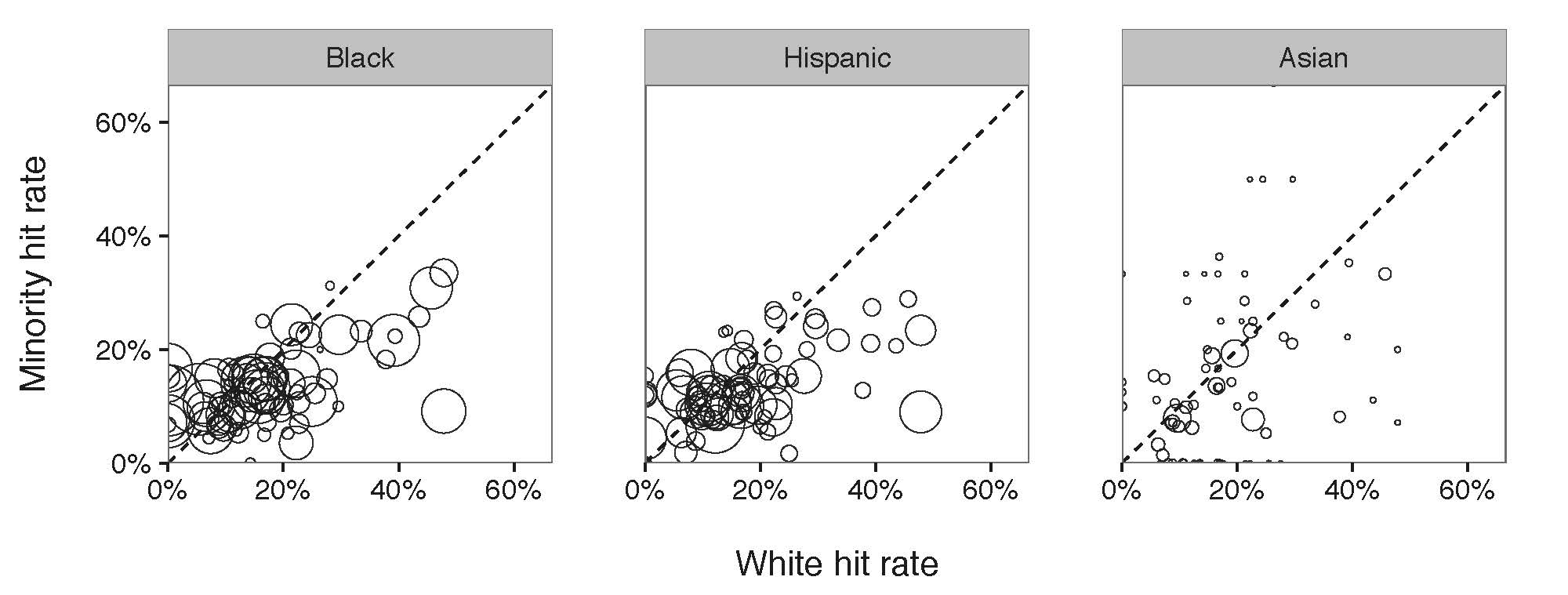
Figure 2: Results of outcome test on a department-by-department basis. Each circle in the diagram compares the corresponding department hit rates. Different with benchmark test, the outcome test showed that the majority of the police departments had a subtle discrimination against Black and Hispanic.
Similar to the Figure 1, if there is no discrimination, all the points in the diagram are expected to locate on the diagonal line. But if they are clustered below the line, we conclude that the hit rate of the minority is below that of White group, leading to a discrimination against the minority. According to Figure 2, the hit rate of Black and Hispanic are below the diagonal line, from which locate a discrimination against Black and Hispanic. Still, no discrimination shows against Asian drivers.
Threshold
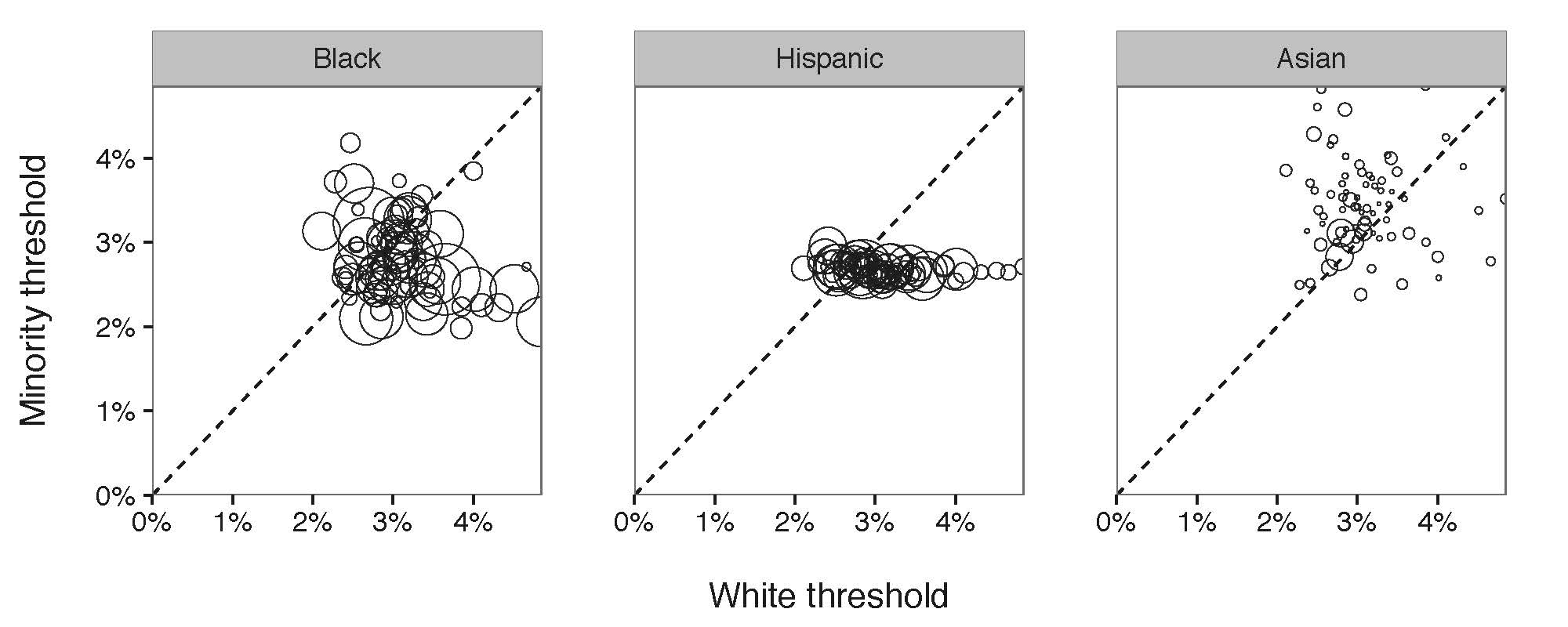
Figure 3: Diagram of the threshold tested computed on the 76 police departments in New York Island Area. Similarly, each point refers to the numbers of minorities stopped by each department. Most of the departments stopped Black with a lower threshold compared to White, meaning that a discrimination exists.
Out of expectation, in the Hispanic/White threshold diagram, all of the departments had almost the same threshold for Hispanic indicating that they were consistent while stopping Hispanic. However, their consistency still indicates a racial bias while having a lower search threshold for Hispanic.
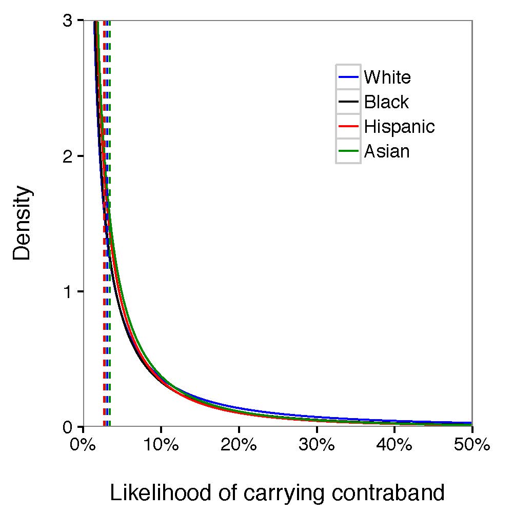
Figure 4: Averaging the race-specific search threshold and signal distribution among all the departments, we found that the likelihood of carrying contraband from Hispanic and Black was slightly lower than White and Asian given the density, suggestive of discrimination against Black and Hispanic. The gap between those four groups was not clear to claim that police forces were biased during stop and frisk operations.
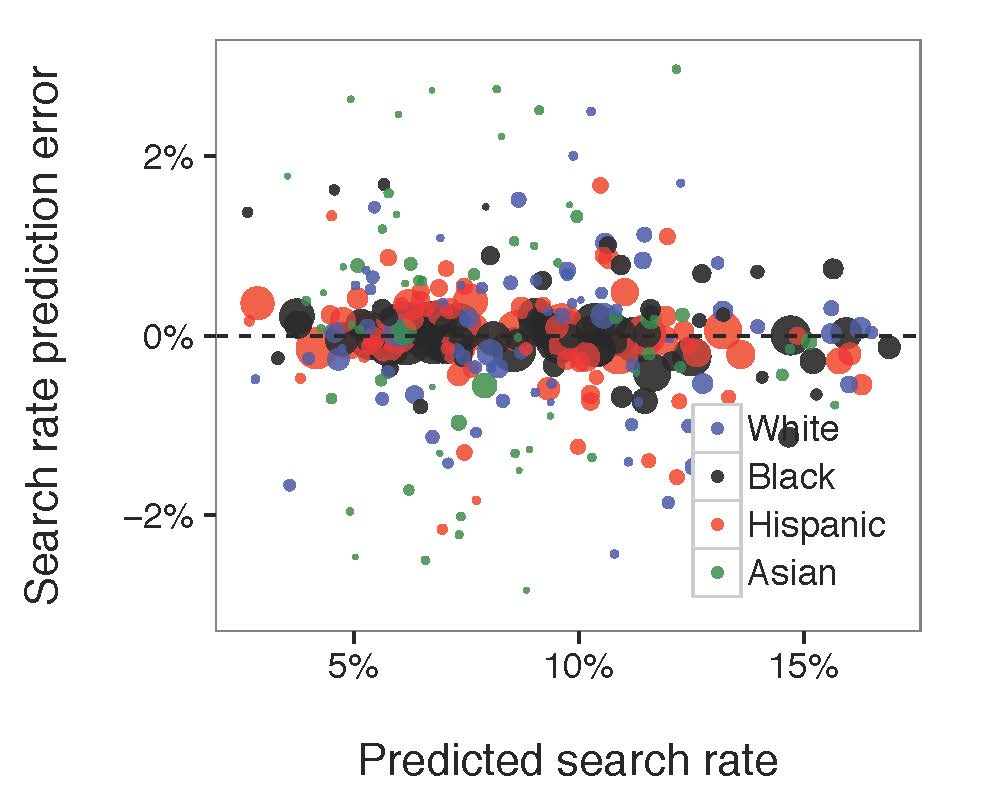
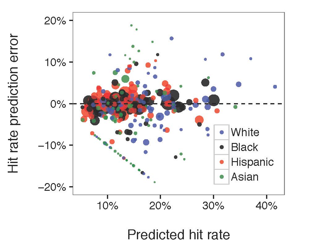
Figure 5: Compared the diagram of predicted search rate, the diagram of predicted hit rate to the actual, observed values. Each circle in the diagram referred to the associated race-paired department. The size of the circle represented the number of stops made by the related police department.
The model fitted well for both search rate and hit rate. No matter how much the search rate/hit rate grows, the prediction error was generally constant. Most of the large bubbles were around the middle line indicating that the model fits the larger groups of department-race pairs well. However, there is a mysterious straight line in the predicted hit rate/ hit rate prediction error chart that might be caused by our buggy data.
Debug Documentation
1 SUM()
Error in eval(substitute(expr), envir, enclos) : ‘sum’ not meaningful for factors.
Variables in data frames are considered as factors. However, the sum function doesn’t take factors as a valid input data type which caused the error while fitting data.
2 Binomial Indexes
“Exception thrown at line 104: binomial_log: Successes variable[231] is 8, but must be in the interval [0, 7]”
In order to find this bug, we tracked the r, n, s, h value of variable[231]. Here is what we found: r[231] = 4, n[231] = 17, s[231] = 7, h[231] = 8. The problem is obvious, the hit (h) count cannot be higher than search (s) count! This made us think about: is any chance in our database that some contrabands found without any search conducted? Fun fact, more than 3000 pieces of observations from more than 660,000 pieces showed without a search, officers still found contraband. Hence, we filtered out the rows with contraband found but without any search conducted and fixed the problem.
Reference: